Assessing the forecastability of a time series
Abir Jameel
- October 17, 2021
Although there are many statistical measures that we can use to assess the predictability of a time series, we will just look at a few that are easier to understand and practical when dealing with large time series datasets.
Coefficient of Variation
The Coefficient of Variation (CoV) means that the more variability that you find in a time series, the more complex it gets to predict. And how do we measure variability in a random variable, the answer is Standard deviation!
In many real-world time series, the variation we see in the time series is dependent on the scale of the time series. Let’s imagine that there are two retail products, A and B. A has a mean monthly sale of 15, while B has 50. If we look at a few real-world examples like this, we will see that if A and B have the same standard deviation, B, which has a higher mean, is much more forecastable than A. To accommodate this phenomenon and to make sure we bring all the time series in a dataset to a common scale, we can use the CoV:
Here, σ is the standard deviation and μ is the mean of the time series.
The CoV is the relative dispersion of data points around the mean, which is much better than looking at the pure standard deviation. The larger the value for the CoV, the worse the predictability of the time series. There is no hard cut-off, but a value of 0.49 is considered a rule of thumb to separate time series that are relatively easier to forecast from the hard ones. But depending on the general hardness of the dataset, we can tweak this cut-off. Something I have found useful is to plot a histogram of CoV values in a dataset and derive cut-offs based on that.
Even though the CoV is widely used in the industry, it suffers from a few key issues:
- It doesn’t consider seasonality. A sine or cosine wave will have a higher CoV than a horizontal line, but we know both are equally predictable.
- It doesn’t consider the trend. A linear trend will make a series have a higher CoV, but we know it is equally predictable like a horizontal line.
- It doesn’t handle negative values in the time series. If you have negative values, it makes the mean smaller, thereby inflating the CoV.
To overcome these shortcomings, there are other derived measures.
Residual variability
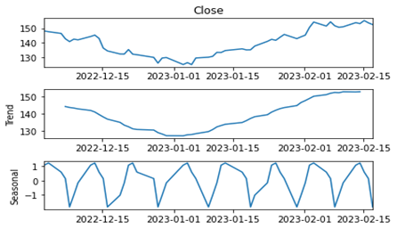
The thought behind residual variability (RV) is to try and measure the same kind of variability that we were trying to capture with the CoV but without the shortcomings. I was brainstorming on ways to avoid the problems of using the CoV, typically the seasonality issue, and was applying the CoV to the residuals after seasonal decomposition. The residuals would have a few negative values and the CoV wouldn’t work well. Stefan de Kok, who is a thought leader in demand forecasting and probabilistic forecasting, suggested using the mean of the original actuals, which worked.
To calculate RV, you must perform the following steps:
- Perform seasonal decomposition.
- Calculate the standard deviation of the residuals or the irregular component.
- Divide the standard deviation by the mean of the original observed values (before decomposition).

The key assumption here is that seasonality and trend are components that can be predicted. Therefore, our assessment of the predictability of a time series should only look at the variability of the residuals. So, higher the residual variability the complex it gets to model and forecast the time series and lower the value means simpler it is to forecast it.
About Author
Abir Jameel

Time Series and its components
Recent Comments
Categories
Archives
- May 2024 (1)
- January 2024 (1)
- October 2023 (1)
- July 2022 (1)
- October 2021 (2)
Categories
- Advanced 1
- Beginner 2
- Intermediate 2
- Tech 2

