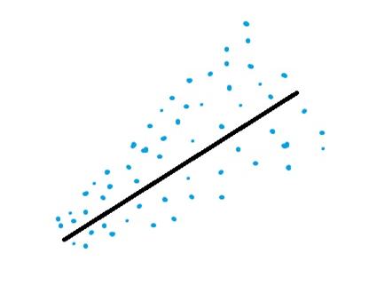
Despite having a scary name, heteroscedasticity is a simple enough concept. It is derived from ancient Greek, where hetero means different and skedasis means dispersion. heteroscedasticity is defined when the variability of a variable is different across another variable. In the context of a time series, we say a time series is heteroscedastic when the variability or dispersion of the time series varies with time. For instance, let’s think about the spending of a household through the years. In these years, this household went from being poor to middle class and finally upper middle class. When the household was poor, the spending was less and only on essentials, and because of that, the variability in spending was less. But as they approached upper middle class, the household could afford luxuries, which created spikes in the time series and therefore higher variability.
Detecting heteroscedasticity
There are many ways to detect heteroscedasticity, but we will be using one of the most popular techniques, known as the White test, proposed by Halbert White in 1980. The White test uses an auxiliary regression task to check for constant variance.
The null hypothesis for White’s test is that the variances for the errors are equal, The alternate hypothesis (the one you’re testing), is that the variances are not equal.
How to remove heteroscedasticity
Log transform
Log transform, as the name suggests, is about applying a logarithm to the time series. There are two main properties of a log transform – variance stabilization and reducing skewness – thereby making the data distribution more normal. And out of these, we are more interested in the first property because that is what combats heteroscedasticity. Log transforms are typically known to reduce the variance of the data and thereby remove heteroscedasticity in the data. Intuitively, we can think of a log transform as something that pulls in the extreme value on the right of the histogram, at the same time stretching back the very low values on the left of the histogram.
Box-Cox transform
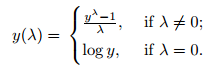
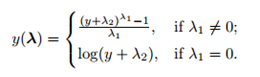
At the core of the Box Cox transformation is an exponent, lambda (λ), which varies from -5 to 5. All values of λ are considered and the optimal value for your data is selected; The “optimal value” is the one which results in the best approximation of a normal distribution curve. The transformation of Y has the form: